Time Series Decomposition
The decomposition of time series data is a statistical method that deconstructs it into notional components. Several decomposition methods exist and the Logi Forecast.Time Period Decomposition element uses "Decomposition Based on Rates of Change".
This is an important technique for all types of time series analysis, especially for seasonal adjustment. It seeks to construct, from an observed time series, a number of component series (that could be used to reconstruct the original by additions or multiplications) where each of these has a certain characteristic or type of behaviour. For example, Monthly or Quarterly economic time series are usually decomposed into:
- a Trend Component T that reflects the long term progression of the series
- a Cyclical Component C that describes repeated but non-periodic fluctuations, possibly caused by the economic cycle
- a Seasonal Component S that reflects seasonality (seasonal variation)
- an Irregular Component I that describes random, irregular influences (or "noise"). Compared to the other components it represents the residuals of the time series.
The equation used in the method is: Y = T * S * C * I
Input Data Requirements
Data should conform to the following requirements:
- Dependent data column data should have Numeric data type
- Dependent data column data should not contain NULL values
- Independent data column should have DateTime or Date data type
- Dataset should be in ascending order by independent data column value
- Forecast Length attribute should be less than original row count (if user defines Forecast Length as more than row count, Forecast Length value will automatically be truncated to 20% of RowCount)
- Source rows count should be not less than season count
Data Validation
It's necessary to check the dataset for inconsistencies before running the forecasting algorithm. "Empty spaces" inside time series are not allowed, a validation process checks the dataset in advance. If an iteration includes more than three "empty spaces", such as "Jan, Feb, July, Aug...", validation returns an error. Otherwise, validations fills missing time periods with the average of the values for the previous and next period. For example, the following dataset,
which is missing data for February:
| Iteration | Source Data |
| January | 10 |
| March | 30 |
| April | 40 |
becomes:
| Iteration | Source Data | Validated Data |
|---|---|---|
| January | 10 | 10 |
| February | 20 | |
| March | 30 | 30 |
| April | 40 | 40 |
Time Series Iteration
Time Series Decomposition requires defined date iteration, which is necessary for the determination of the seasonal component. These date iterations are used:
| Iteration | Season Count | Season Determination |
|---|---|---|
| Hour | 24 | Hour |
| Day | 7 | Day of Week |
| Week | 5 | Week of Month |
| Month | 12 | Month |
| Quarter | 4 | Quarter |
| Year | 1 | No season |
Method Implementation
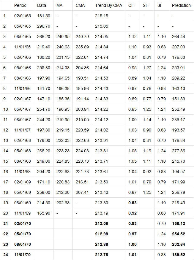
- "Deseasonalizing" the data: Remove short-term fluctuations from the data, so that the longer-term trend and cycle components can be more clearly identified. These short-term fluctuations include both seasonal patterns and irregular variations. They can be removed by calculating an appropriate Moving Average (MA) for the series, which should contain the same number of periods as there are in the seasonality that we want to identify. If the season count is an even number, the moving averages are not really centered in the middle of the seasons. We calculate a Centered Moving Average (CMA) and it represents the deseasonalized data.
- Determine Seasonical Factor (SF), which is the ratio of the actual value to the deseasonalized value.
- Create Season Index (SI) for each season, which is the normalized mean of the seasonal factors for the selected season.
- Estimate Long Term Trend from the deseasonalized data using linear regression.
- The cyclical component of a time series is the extended wavelike movement about the long-term trend. It is measured by the Cycle Factor (CF), which is the ratio of the Centered Moving Average to the Long Term Trend.
- Determine forecast for Cyclical component by using AutoRegression with Order equal to the Count of seasons (use 4 if no season).
- Calculate forecast for time series.
Forecast Calculations Example
The following table displays the calculation used for a forecast, assuming Quarterly data for a 1-year forecast:
Results
As a result of the forecast operation, two new columns will be added to the datalayer. The names of these two columns will be drawn from the element's attributes:
- Forecast Indicator Column ID: this column will contain a boolean flag, set to True if the row contains a forecast value
- Forecast Value Column ID: this column will contain the forecast value for each row of the original dataset
|